We predicted COVID-19 cases with 95% accuracy, this is how we did it
When the first COVID-19 case was discovered in the United States of America (USA) in early march, many believed that the disease would never spread in this country. However, the number of cases have spiked exponentially to 6.5 million and continue to grow each and every day. Despite the existence of many other Machine Learning models out there, Facebook Prophet seems to be one of the most effective models in predicting/forecasting future COVID-19 cases. Most importantly, it automates many of the parameters that require tuning in a time series model. By the end of the article, you will be able to understand what the Facebook Prophet does, and use it to build your own Machine Learning models.
Introduction to Time Series Forecasting with Seasonality
In normal data analysis, the order of observations that are collected is usually irrelevant. However, most of the data collected in the real world has a certain order built into it. This structure can be exploited for better prediction ability by employing a Time Series Model. The first step in analyzing a time series model is identifying and understanding the built-in structure of the data over time. These underlying patterns can be classified into four distinct categories:
- Trend - Long term pattern in the data (easiest to identify).
- Seasonality - Short term patterns that occur within the overall time structure, and repeat indefinitely.
- Cyclical Component - Long term oscillations (big waves) within the overall time structure.
- Noise(Error) - Random changes occuring in the overall time structure (unlikely to be repeated).
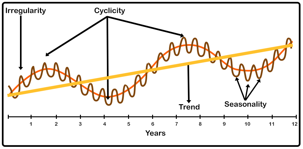 $$\text{Figure 1: Time Series Components}$$
The second step is to check the underlying assumptions:
- Stationarity - This means that the series are normally distributed and the mean and variance are constant over a long time period.
- Uncorrelated Random Error - We assume that the error term is randomly distributed and the mean and variance are constant over a time period.
- No outliers - This one is self-explanatory.
- Random shocks - If shocks are present, they are assumed to be randomly distributed with a mean of 0 and a constant variance.
Once these assumptions are met (or not too badly violated), we can start building our Time Series Model. The model description is as follows:
- Notation for Time Series Data
- $Y_T$ = value of $Y$ in period $t$
- Data set: $Y_1,...,Y_T = T$ observations on the time series random variable $Y$
- We consider only consecutive, evenly-spaced observations. Missing data can cause technical problems, but that can be dealt with in a systematic manner.
- The first lag in a time series $Y_T$ is $Y_{t-1}$; its $j^{th}$ lag is $Y_{t-j}$.
- The first difference of a series, $\Delta Y_t$, is its change between periods $t-1$ and t, that is, $\Delta Y_t = Y_t - Y_{t-1}$
- If we assume that $Y_t$ is stationary, a natural starting point for a forecasting model is to use past values of $Y$ (that is, $Y_{t-1},Y_{t-2},...$) to forecast $Y_t$.
- An autoregression is a regression model in which $Y_t$ is regressed against its own lagged values.
- The number of lags used as regressors is called the order of the autoregression.
- In a first order autoregression, $Y_t$ is regressed against $Y_{t-1}$
- In a $p^{th}$ order autoregression, $Y_t$ is regressed against $Y_{t-1}, Y_{t-2}, ... , Y_{t-p}$.
Let's look at a First Order Autoregressive Model (AR(1)) Model:
- $Y_t = \beta_0 + \beta_1Y_{t-1} + \mu_t$
- The AR(1) model can be estimated by Ordinary Linear Squares regression of $Y_t$ against $Y_{t-1}$.
- Testing $\beta_1 = 0$ vs. $\beta_1 \neq 0$ provides a test of the hypothesis that $Y_{t-1}$ is not useful in forecasting $Y_{t}$.
- A $p^{th}$ order autoregression follows a similar process.
Let's look at some Forecasting Terminology and Notation:
- Predicted values are "in-sample".
- Forecasts are "out-of-sample" - in the future.
- Notation
- $Y_{T+1|T} =$ forecast of $Y_{T+1}$ based on $Y_T,Y_{T-1},...,$ using the population (true unknown) coefficients
- $\hat{Y}_{T+1|T}$ = forecast of $Y_{T+1}$ based on $Y_T,Y_{T-1},...,$ using the estimated coefficients, which are estimated using data through period $T$.
- For an AR(1)
- $Y_{T+1|T} = \beta_0 + \beta_1Y_T$
- $\hat{Y}_{T+1|T} = \hat{\beta}_0 + \hat{\beta}_1Y_T$, where $\hat{\beta}_0$ and $\hat{\beta}_1$ are estimated using data through period $T$.
- A similar procedure is employed for a $p^{th}$ order autoregression.
- Forecast errors vs. residuals
- Forecast error is "out of sample" because the value of $Y_{T+1}$ isn't used in the estimation of the regression coefficients.
- forecast error $= Y_{T+1} - \hat{Y}_{T+1|T}$
- A residual is "in sample" error.
- Exact same formula as the forecast error but the values are used in the estimation of the regression coefficients.
- Forecast error is "out of sample" because the value of $Y_{T+1}$ isn't used in the estimation of the regression coefficients.
Introduction to Facebook Prophet Model
The Facebook Prophet model is an accurate, fast modular regression model that often performs really well with just the default parameters. The python library, fbprophet, comes with mulitiple functionalities. Analysts, often, have to select the components that are relevant to their particular problem. We are going to modify a few of the existing components to fit our needs for this COVID-19 study.
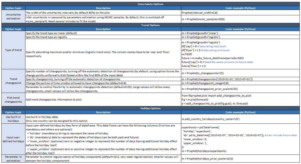 $$\text{Figure 2: fbprophet functions in Python}$$
We shall give a brief introduction to each and every component in this graphic, before we apply the model to our analysis.
The Prophet Forecasting Model
The main model equation (broken into individual components) is:
- $y(t) = g(t) + s(t) + h(t) + \varepsilon(t)$
- $g(t)$: piecewise linear or logistic growth curve
- $s(t)$: periodic changes (e.g. weekly/yearly seasonality)
- $h(t)$: effects of holidays (user provided) with irregular schedules
- $\varepsilon(t)$: error term accounts for any unusual changes not accommodated by the model
Using time as a regressor, Prophet is trying to fit several linear and non-linear functions of time as components. Modeling seasonality as an additive component is the same approach taken by exponential smoothing in Holt-Winters Technique. Prophet is framing the forecasting problem as a curve-fitting exercise rather than looking explicitly at the time based dependence of each observation within a time series.
Python's fbprophet Library's Functionality
Referring back to Figure 2, we can see that the Facebook Prophet model can utilize Markov Chain Monte Carlo (MCMC) to do the uncertainty interval estimation (error terms). This method is used for a Bayesian Statistical approach, but we are not going to apply that to our study. The default uncertainty interval is $80\%$. However, we chose to change that to $95\%$, because that is a commonly used significance level. We used a linear trend (default) for the United States Data because logistic trends are usually reserved for binary data.
Additionally, one advantage of Facebook Prophet is that it automatically discovers changes in trends, and tries to account for it in your analysis. We are not going to make any changes to the default functionality in this part. Facebook Prophet also has built in holidays, and you can input your own holidays, but we chose not to use that for our study. We also didn't use the parameter in estimation to control the impact of the holidays.
Setting up our Facebook Prophet Analysis (USA COVID-19 Data)
Checking Directory
!ls
!pwd
Importing all the required packages
import numpy as np
import pandas as pd
from fbprophet import Prophet
from fbprophet.plot import plot_plotly, plot_components_plotly
from fbprophet.diagnostics import cross_validation
from fbprophet.diagnostics import performance_metrics
from fbprophet.plot import plot_cross_validation_metric
Processing the Raw Data
stay_at_home_df = pd.read_csv("https://covid.ourworldindata.org/data/owid-covid-data.csv")
stay_at_home_df.head()
stay_at_home_df.columns
cleaned_stay_at_home_df = stay_at_home_df[['location','date','total_cases','total_tests','stringency_index','positive_rate','total_deaths']]
cleaned_stay_at_home_df
cleaned_stay_at_home_df['cases_per_tests_ratio'] = cleaned_stay_at_home_df['total_cases']/cleaned_stay_at_home_df['total_tests']
cleaned_stay_at_home_df
cleaned_stay_at_home_df.dtypes
groupby_location_df = cleaned_stay_at_home_df.groupby('location',as_index=False)
separated_location_df = dict(iter(groupby_location_df))
us_covid_df = separated_location_df['United States']
Setting up for our Facebook Prophet Time Series Analysis
def plot_metrics(forecast_cv,location, imgname):
    mse_plot = plot_cross_validation_metric(forecast_cv, metric = 'mse')
    mse_plot.suptitle(f'{location}_mse_{imgname}',y=0.95)
    mse_plot.savefig(f'./Seasonality_Comparison/{location}_mse_{imgname}')

    rmse_plot =plot_cross_validation_metric(forecast_cv, metric = 'rmse')
    rmse_plot.suptitle(f'{location}_rmse_{imgname}',y=0.95)
    rmse_plot.savefig(f'./Seasonality_Comparison/{location}_rmse_{imgname}')

    mae_plot = plot_cross_validation_metric(forecast_cv, metric = 'mae')
    mae_plot.suptitle(f'{location}_mae_{imgname}',y=0.95)
    mae_plot.savefig(f'./Seasonality_Comparison/{location}_mae_{imgname}')

    mape_plot = plot_cross_validation_metric(forecast_cv, metric = 'mape')
    mae_plot.suptitle(f'{location}_mape_{imgname}',y=0.95)
    mae_plot.savefig(f'./Seasonality_Comparison/{location}_mape_{imgname}')


def plot_forecast(forecast,m,location,img_name):
    forecastplot = m.plot(forecast)
    forecastplot.suptitle(f'{location}_forecast_{img_name}',y=0.95)
    forecastplot.savefig(f'./Seasonality_Comparison/{location}_forecast_{img_name}')

    plot_components = m.plot_components(forecast)
    plot_components.suptitle(f'{location}_components_{img_name}',y=0.95)
    plot_components.savefig(f'./Seasonality_Comparison/{location}_components_{img_name}')


def prophet_predicts(location_df,location, yearly_seasonality, weekly_seasonality):
    print(location_df.columns)
    num_rows = str(location_df.shape[0] - 31) + ' days'
    prophet_df = location_df[['date','total_cases']]
    prophet_df = prophet_df.rename(columns={'date':'ds','total_cases': 'y'})
    m = Prophet(interval_width = 0.95, yearly_seasonality = yearly_seasonality, weekly_seasonality = weekly_seasonality)
    m.fit(prophet_df)
    future = m.make_future_dataframe(periods=30)
    forecast = m.predict(future)
    forecast_cv = cross_validation(m, initial = num_rows, period = '30 days', horizon = '30 days' ) # of rows - 31 days

    img_name = 'daily.png'
    if(yearly_seasonality):
        img_name = 'yearly_' + img_name

    if(weekly_seasonality):
        img_name = 'weekly_' + img_name

    plot_forecast(forecast,m, location, img_name)
    plot_metrics(forecast_cv, location, img_name)
Results of our analysis
prophet_predicts(us_covid_df, 'United States', yearly_seasonality = True, weekly_seasonality = False)
prophet_predicts(us_covid_df, 'United States', yearly_seasonality = False, weekly_seasonality = False)
prophet_predicts(us_covid_df, 'United States', yearly_seasonality = False, weekly_seasonality = True)
prophet_predicts(us_covid_df, 'United States', yearly_seasonality = True,  weekly_seasonality = True)
Types of Analysis:
In our study, we tested four different model types within Facebook Prophet. Each model type had a different seasonality parameter. Facebook Prophet always has daily seasonality by default, but we added on yearly, and weekly seasonlity from our end. We shall discuss the forecast graphs, and the model accuracies given by varying seasonality types.
Forecast Graphs and Model Accuracy
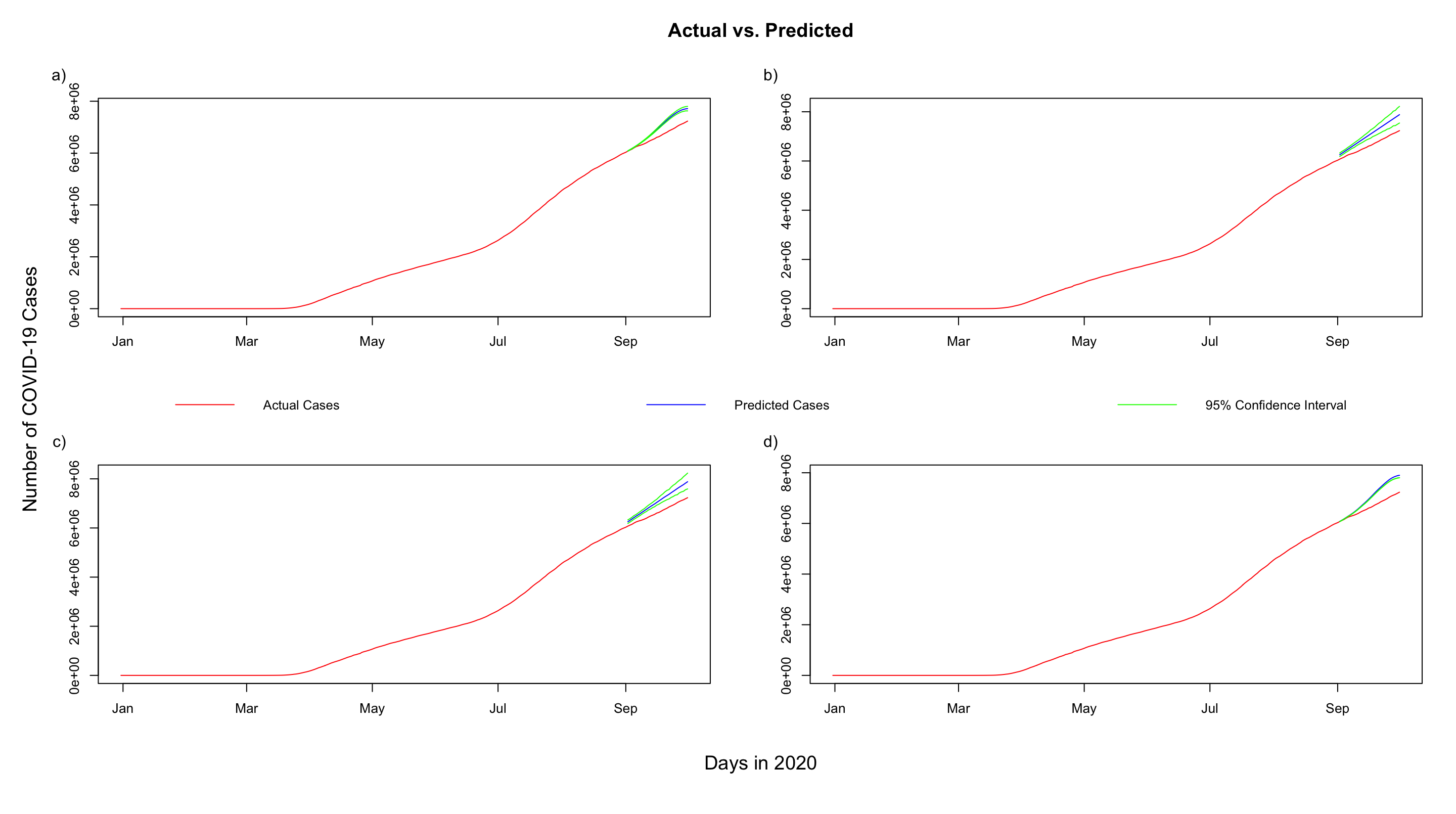 $$\text{Figure 3: a) Yearly & Daily Seasonality. b) Daily Seasonality. c) Weekly & Daily Seasonality. d) Yearly, Weekly & Daily Seasonality.}$$
| Model Type | Model Accuracy |
|---|---|
| Yearly & Daily Seasonality | $95.5585\%$ |
| Daily Seasonality | $93.5955\%$ |
| Weekly & Daily Seasonality | $93.5983\%$ |
| Yearly, Weekly & Daily Seasonality | $94.5314\%$ |
From these results, we can clearly see that Yearly and Daily Seasonality performs marginally better than all the other models. However, even a 4-5% error rate is a lot when you consider the scale of our data. We are overestimating the number of COVID-19 cases in all the models. Our models are predicting 7.8 million cases by the beginning of October. We are currenlty at 7.4 million cases. This phenomenon might be occuring because the model hasn't detected the change in trend because it is a recent event. We believe that more training values will cause the models to detect the change and give more accurate predictions. Our next articles will cover the ARIMA Time Series Model, and the LSTM Neural Network Model.